A primer on Unsupervised Domain Adaptation
An introduction to popular practices in UDA.
AI has ushered us into a new era of a technological revolution. From detecting brain tumours to autonomous navigation, AI has founded its way into our everyday lives in a very short amount of time, so much so that there is a consensus that AI will soon take over the world. However, that possibility is still far into the future. At the heart of such tremendous advancement in AI are the Deep Learning (DL) algorithms. DL is a branch of machine learning algorithms that can approximate any function over a finite set of iterations. However, there are two limitations to this wonder algorithm. Firstly, they need a lot of hand-annotated training examples and secondly, they do not generalise well to examples outside of the training data. Although the first problem can be solved to a certain extent by synthetically generating training pairs, it is the issue with models not generalizing to out of distribution data that is more troublesome. For example, an autonomous navigation DL model trained on US road images will not work in the Indian setting. For a model to work on Indian roads we will need to collect and annotate huge amounts of data from Indian roads and train a model from scratch which is both expensive and time-consuming.
Introduction
The main reason behind a DL model’s poor generalisability is the difference in the target and source data distribution which is also known as domain shift. A workaround will be to fine-tune a pre-trained model on a target task by annotating only a small amount of the target data. However, the amount of annotated data required for finetuning depends on the task at hand. For example, sequences based tasks like Machine Translation or Speech Transcription require a lot of effort and labelling even a small portion of the dataset can take a significant amount of time and effort. Another way would be to train the model in an unsupervised manner such that it learns to focus on features that are domain invariant. Such methods fall under the umbrella of unsupervised domain adaptation (UDA) and it is something that we will discuss in much more detail in this blog post.
Formally, Domain Adaptation can be defined as a set of methods or practices that enable the model trained on a “source” data to perform well on a “target” data distribution. Finetuning can also be considered as a domain adaptation technique. However, in this blog post, we will look only at those domain adaptation techniques that do not require any labels in the target domain i.e. unsupervised domain adaptation.
We will look at several unsupervised domain adaptation techniques. This post can be thought of as a mini-literature survey meant to initiate the readers on the topic of UDA. Although there can be various approaches towards solving UDA, I have focused on two of the most common techniques: (a) Adversarial (b) Self-Supervised. For both approaches, I have picked some of the most relevant papers and tried to explain them as concisely as possible.
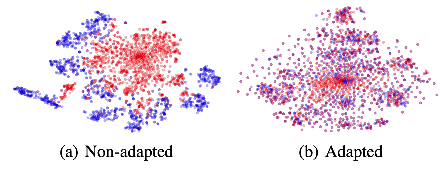
Fig.1. shows the t-SNE visualization of CNN features for (a) before and (b) after adaptation is performed on CNN features. The Bluepoints correspond to source domain examples and the red data points refer to target examples. (Image source: Ganin et al., 2015)
Adversarial Domain adaptation
UDA aims to align the source and target features such that they are indistinguishable from the classifier. There are several possible ways one can achieve this. Sun and Saenko minimise the first and second-order moments for the source and target data. Another way is via maximizing the mean discrepancy of target and source feature distribution proposed by Long and Wang. However, one of the most common and intuitive ways to align source and target data distribution is via adversarial learning.
Gradient Reversal
Ganin et al., 2016 was one of the earliest works to explore domain adaptation via adversarial learning. The underlying principle is very simple. The authors formulate the problem as a classification task where the classifier should be able to perform well not just on source features but also on the target features. They define a feed-forward architecture that should be able to predict not just the label of the input but also its domain label i.e. whether it belongs to the source or target category.
They decompose such a mapping into three parts (refer Fig.2.):
- $G_f(a\ feature\ extarctor)$ with parameters $\theta_f$ which maps the input $x$ into a $D$-dimensional feature vector ($f$)
- $G_y(label\ predictor)$ with parameters $\theta_y$ which maps the feature vector $f$ to a label space $y$.
- $G_d$ with parameters $\theta_d$, which maps the same feature vector $f$ to the domain label $d$.
Like any feedforward network, they optimise the feature extractor and label predictor to minimize the label prediction loss on source labels. At the same time, they want both the source and target feature distributions to be close to each other so that accuracy on the target domain remains same as the accuarcy on the source domain. To learn domain invariant features, during training time, the authors pose the optimization problem such that $\theta_f$ seeks to maximize the loss of the domain classifier, while $\theta_d$ of the domain classifier tries to minimize the loss of the domain classifier.
\begin{equation} \begin{array}{l} E(\theta_f, \theta_y, \theta_d)=\sum_{l=1 \atop d_{i}=0}^{N} L_{y}\left(\theta_{f}, \theta_{y}\right)-\lambda \sum_{i=1}^{N} L_{d}\left(\theta_{f}, \theta_{d})\right. \end{array} \end{equation}
Equation 1 represents the overall loss function. Here $L_y$ is the classifier loss, $L_d$ is the domain classifier loss. Optimal parameters will result in a saddle point.
\begin{equation}
(\theta_f, \theta_y) = arg\ min E(\theta_f, \theta_y, \theta_d)
\end{equation}
\begin{equation} \theta_d = arg\ max E(\theta_f, \theta_y, \theta_d) \end{equation}
The above optimization problem can be thought of as a min-max game between the feature extractor and the domain classifier. The $\theta_d$ of the domain classifier tries to minimize the domain classification loss while $\theta_f$ of the feature extractor tries to fool the domain discriminator, thereby maximizing the domain classification loss. On the other hand, since we want to learn discriminative features for both source and target samples, $\theta_f$ and $\theta_y$ seek to minimize the label prediction loss.
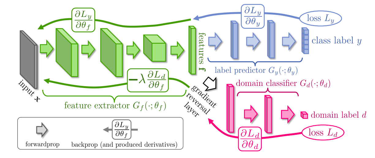
Fig.2. The architecture proposed by Ganin et al. 2015. The figure highlights the feature extractor, the label predictor and the domain classifier. Gradient reversal is achieved by multiplying the domain classifier gradient w.r.t with a negative constant. Gradient reversal ensures that the source and target feature distributions lie close to each other. (Image source Ganin et al. 2015)
Intuition behind the gradient reversal layer
Without the gradient reversal layer, the network will behave like a traditional feed-forward network. The network will be good at predicting the class label as well as the domain labels. However, we do not want that. We want the network to predict the class labels correctly but only on features that are domain invariant. To obtain domain invariant features, the authors propose to reverse the gradients coming from the domain classifier and going into the feature extractor. Gradient reversal is achieved by multiplying $\frac{\partial L_d}{\partial \theta_f}$ with a negative constant $\lambda$. Multiplying $\frac{\partial L_d}{\partial \theta_f}$ and not $\frac{\partial L_d}{\partial \theta_d}$ with a negative constant enforces a min-max game between the feature extarctor and the domain discriminator, where the feature extractor tries to learn features which can fool the disciminator, thus maximizing the domain prediction loss.
Self-supervised Domain Adaptation
Although adversarial domain adaptation works quite well, they pose the training objective as a min-max training problem which is known to be quite difficult to solve. The training often does not converge and if it does, it converges to a bad local maximum. One also need to balance the two sets of parameters (for generator and discriminator) so that one does not dominate the other. Self-supervised domain-adaptation avoids the adversarial game altogether and seeks to align the source and target features by training a model on an auxiliary task in both domains.
Rotation, Flip and Patch prediction
Although, one can choose a variety of auxiliary tasks such as Image colourization or image in-painting, Sun e al., 2019 verified empirically that such pixel prediction/reconstruction task is ill-suited for domain adaptation as they induce domain separation. They showed that classification tasks which predict labels based on label structure such as Rotation prediction, Flip Prediction and Patch location prediction are more suited for domain adaptation.
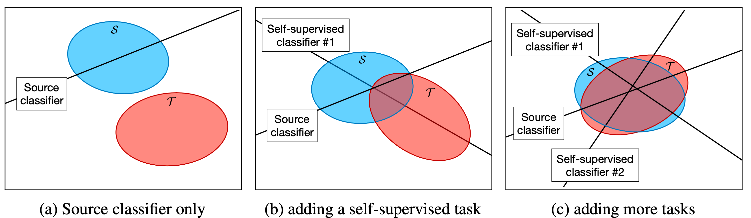
Fig. 3. shows how the source and target features are aligned on a shared feature space (a) before and (b) after training the model on a single auxiliary task which subsequently leads to alignment of domains along a particular direction. (c) highlights when we train the model on multiple self-supervised tasks which further aligns the domains along with multiple directions. (Image source Sun et al., 2019)
They proposed a method where in addition to the supervised classification loss on source data points $L_0$, they also had a set of $K$ self-supervised tasks, each with its separate loss function $L_k$ where $k=1\dots,K$. All the task-specific heads $h_k$ for $k=0\dots K$, share a common feature extractor $\phi$ as shown in Fig.3. where $\phi$ is a convolutional neural network and each $h_k$ is a linear layer.
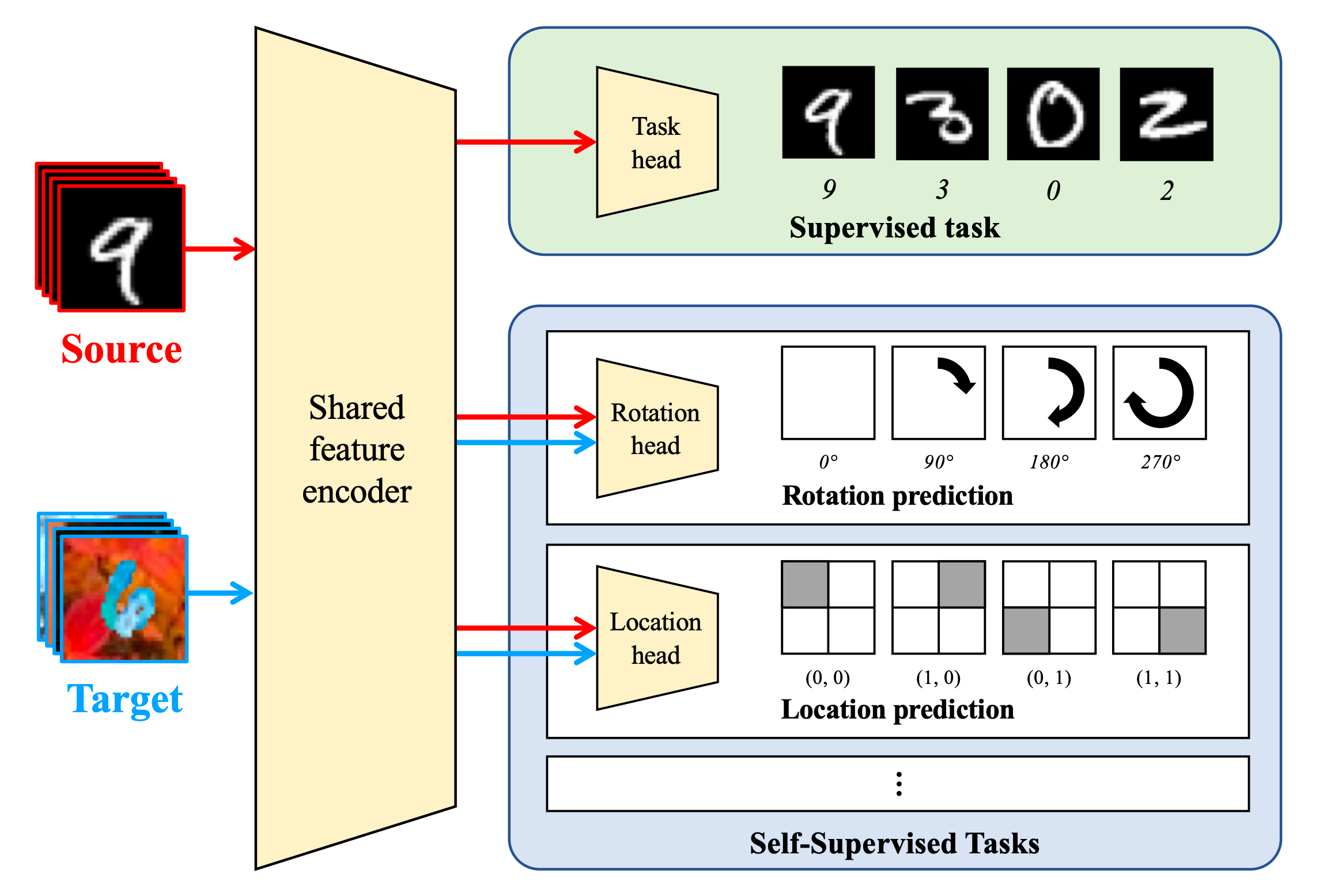
Fig. 3. shows the architecture proposed by Sun et al., 2019. The network is trained jointly on the source and target examples. Each head corresponds to a separate task either supervised or self-supervised and has its separate loss function associated with it. All the heads share a common feature extractor, which learns to align feature distributions. (Image source Sun et al., 2019)
So if $S = {(x_i, y_i), i=1\dots m}$ is the labeled source data and $T = {(x_i), i = 1 \dots n}$ is the unlabelled target data then the overall loss function can be written as:
\begin{equation}
L = \sum L_0(S;\phi,h_0) + \sum_{k=1}^{K}L_k(S,T;\phi,h_k)
\end{equation}
Here, we see that the term $L_k$ unlike the term $L_0$ takes both the source and target examples which is crucial for inducing feature alignment. In their paper, the authors set $K=3$, where the auxiliary tasks are the ones mentioned above.
Jigsaw puzzles
Carlucci et al., 2019 via a similar approach showed that domain adaptation could be achieved by when a model is trained to solve jigsaw puzzles i.e. recovering an image from its shuffled parts for both source and target examples. The authors argue that solving the jigsaw puzzle as a side objective to the real classification task act not only as a regularisation measure but also aids in feature adaptation. The overall loss function is similar to equation 4 with being equal to
Open Set Domain Adaptation
The examples that we have seen till now belong to the closed set domain adaptation where there is a complete overlap between the source and target labels. However, in real-world applications, it will be difficult to say a priori whether our task will have the same set of labels as our source task. In many practical scenarios, our target task may have labels that are unseen in the source task. In such cases, the closed-set distribution matching algorithms will try to align the source and target domains irrespective of the fact whether the source and target domains share the same label space or not. This will cause the data samples with the “unknown” classes in the target domain to also become aligned with the “known” classes in the source domain which will deteriorate the performance of the model and lead to negative transfer (a phenomenon where an adapted model performs poorly as compared to a model which was trained exclusively on source data). Thus it becomes important to identify a boundary between the known and unknown samples and apply adaptation only on those samples which have the same classes as the source.
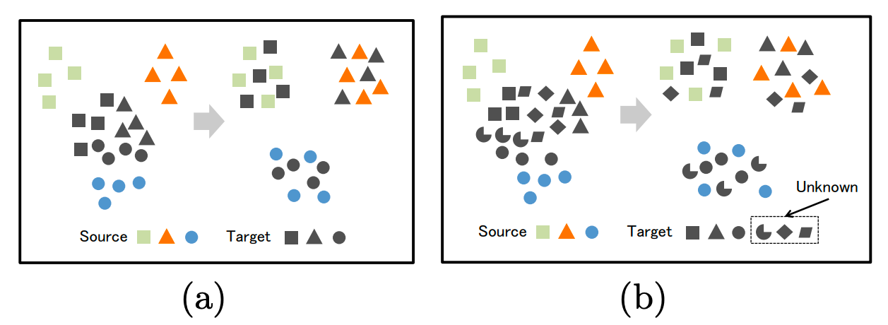
Fig.4. (a) Closed set domain adaptation with distribution matching algorithm. (b) Open set domain adaptation with distribution matching algorithm. The unknown classes in the target domain are aligned with the known classes of the source domain. (Image source Saito et al., 2018)
Adversarial Open Set Domain adaptation
Open set domain adaptation was proposed Busto et al., 2017 where the target and source domain categories do not overlap completely. The main idea behind their solution was to be able to draw a decision boundary that can differentiate between the target samples belonging to either the “known” or “unknown” class and classify correctly only the “known” class target samples. To do so, they add unknown source samples to the known source samples to learn a mapping that can classify the target samples to either one of the “known” classes or the “unknown” class. Although the algorithms do a decent job, collecting unknown source samples can be a challenging task since we must collect a diverse set of unknown samples to define what is unknown.
Gradient Reversal via Back-propagation
Saito et al., 2018 proposed a method for open set DA which involved no “unknown” source samples. Their method is similar to the one proposed by Ganin et al., 2016 with a few tweaks to also consider the unknown target samples. Fig. 5. shows the architecture used in their paper.
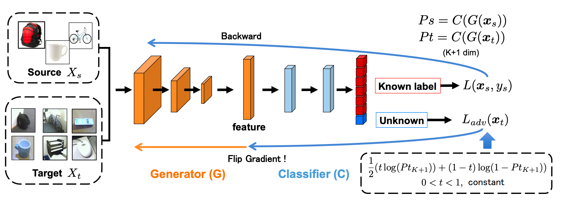
Fig. 5. Network architecture proposed by Saito et al., 2018. The above architecture consists of a feature generator (G) and a classifier (C) which can classify a data point into K+1 (K known classes and an unknown class). The proposed method makes use of a Gradient Reversal Layer similar to the one proposed by Ganin et al., 2016. (Image source Saito et al., 2018)
The main objective as mentioned earlier is to correctly classify the “known” target samples and differentiate the “unknown” target from class samples from the “known”. To achieve this, one needs to create a decision boundary that can correctly separate the “unknown from the known samples. However, since there is no label information for the target samples, the authors propose to come up with a pseudo decision boundary by training the classifier to classify all the target samples as belonging to the “unknown” class. The role of the feature generator would then be to fool the classifier into believing that the target samples comes from the source domain.
However, there is a small catch in this. In the traditional sense, if we were to train a classifier to classify the target sample as unknown, then it would be as good as saying that we want the output probability of the target sample to be $p(x_t) = 1$. In such a case, for the generator to deceive the classifier, it should align the target samples completely with the source samples. The generator will try to decrease the probability for the unknown class which will ultimately lead to negative transfer.
To combat the above situation, the authors propose that the classifier should output a probability $t$ instead of 1, where $0 < t < 1 $. The generator can choose to either increase or decrease the value of the output probability of an unknown sample and thereby maximize the classifier error. Now, this has two implications. If the generator chooses to decrease output probability lower than , then it essentially means that the target sample is aligned with the source class. Similarly, if output probability is increase to a value greater than , then it means that the sample must be rejected.
Equation 5 refers to the cross-entropy loss used to train the model to identify the source data into one of the known classes.
\begin{equation} L_s(x_s, y_s) = -log(p(y = y_s|x_s)) \end{equation}
For training a classifier to learn a decision boundry seperating the known and unknown classes, the authors propose binary cross-entropy loss.
\begin{equation}
L_{adv}(x_t) = -tlog(p(y = K + 1|x_t)) - (1 - t)log(1 - p(y = K + 1|x_t))
\end{equation}
Where $t$ is set as $0.5$.
The overall training objective becomes
\begin{equation} L_C = min(L_s(x_s, y_s) + L_{adv}(x_t, y_t) \end{equation}
\begin{equation} L_G = min(L_s(x_s, y_s) - L_{adv}(x_t, y_t) \end{equation}
Intuition
But wait a minute. How does the feature extractor choose? I mean it is possible that the feature extractor mistakenly assumes that a particular “unknown” target sample belonging to the “known” class. In such a case, the feature extractor can decide to manipulate its feature vector such that the classifier outputs a probability score of less than . In such a case the unknown class target sample becomes aligned to the known source sample which will then lead to negative transfer.
However, the authors claim that the feature extractor can recognize the distance between each target sample and the boundary between the known and the unknown class. Thus, for the target samples which are similar to the source samples, the extractor tries to align them to the known source samples and for the different ones it tries to separate them from the known class.
Self-supervised Open set Domain Adaptation
Now that we have looked at adversarial open set domain adaptation, it only makes sense to look at its self-supervised counterpart. Saito et al., 2020 took a leaf out of a prototype-based few-shot learning paradigm and propose a technique called “Neighbourhood Clustering (NC)”. In NC each target sample is either aligned to the “known” class prototype in the source or its neighbour in the target. NC encourages the target samples to be well clustered. However, we also want to know which target samples should be aligned with the source and which target samples should be rejected as “unknown”. It is always possible for a target sample belonging to a “known” class to be clustered around another target sample of the same class instead of the source prototype. Thus, in addition to NC, the authors also propose an “Entropy Separation loss” (ES) to draw a decision boundary to separate the “known” and the “unknown” class samples.
Neighbourhood Clustering and Entropy Separation
In NC, the authors try to minimize the entropy of a target samples’ similarity distribution to other target samples and source prototype. By doing so, the authors claim that the target sample will either move to a nearby target sample or a source prototype.
To do so, the authors first calculate the similarity of each target point to all the other target samples and the class prototypes for each mini-batch of target features. In the paper, the class prototypes are the weight vectors of the last fully connected layer of the network trained to classify the source data points.
Thus, if $N_t$ denotes the number of target examples and K denotes the number of classes, then $V \in R^{N_t \times d}$ denotes the memory bank containing all the target features and $F \in R^{(N_t + K) \times d}$ denotes all the feature vectors in the memory bank and the prototype vectors where $d$ is the dimension of last linear layer.
\begin{equation} V = [V_1, V_2 \dots V_{N_t}] \end{equation}
\begin{equation} F = [V_1, V_2, \dots V_{N_t}, w_1, w2 \dots w_k] \end{equation}
Since the authors calculate the similarity of feature vectors at a mini-batch level, they employ $V$ to store the features which are not present in the mini-batch. Let $f_i$ denote the features in the mini-batch and $F_j$ denote the $j$-th term in $F$, then the similarity matrix for all the features in the mini-batch can be obtained by:
\begin{equation} p_{i,j} = \frac{exp(F_j^T f_i/\tau)}{Z_i} \end{equation}
\begin{equation} Z_i = \sum_{j=1, j \ne i}^{N_t + K} exp(F_{j}^T f_i/\tau) \end{equation}
where, $\tau$ is the temperature parameter, which controls the number of neighbours for each sample.
The entropy is then calculated by
\begin{equation} L_{nc} = -\frac{1}{B_t}\sum_{i \in B_t} \sum_{j=1,j \ne i}^{N_t + K}p_{i,j}log(p_{i,j}) \end{equation}
Here, $B_t$ refers to all target sample indices in the mini-batch.
The authors make use of the entropy of the classifier’s output to separate the known from the unknown target samples. The intuition behind this is that “unknown” target samples are likely to have higher entropy since they do not share any common features with the “known” source classes.
The authors define a threshold boundry $\gamma$ and try to maximize the distance between the entropy and the threshold which is defined as $H(p) - \gamma$. They assume $\gamma = \frac{log(K)}{2}$, $K$ being the number of classes. The value is chosen empirically. The authors further claim that the value of threshold is ambiguous and can change due to domain shift. Therefore, they introduce a confidence parameter $m$ such that the final form becomes.
\begin{equation} L_{es} = \frac{1}{|B_t|}\sum_{i \in B_t}L_{es}(p_i) \end{equation}
\begin{equation}
L_{es}(p_i) = \begin{cases}
-|H(p_i) - \gamma| & |H(p_i) - \gamma|> m
0 & otherwise
\end{cases}
\end{equation}
The confidence parameter $m$ allows seperation loss only for the confident samples. Thus when $H(p) - \gamma$ is sufficiently large, the network is cofident about a target sample belonging to “known” or “unknown” class.
The final loss function then becomes
\begin{equation} L = L_{cls} + \lambda(L_{nc} + L_{es}) \end{equation}
where $L_{cls}$ is the classifier loss on source samples and $\lambda$ is a weight parameter.
Category-Agnostic Clusters for Open-Set Domain Adaptation
Till now in open domain set domain adaptation we learn a binary classifier to classify a target sample into one of the many “known” source classes or categorize them as belonging to an “unknown” class. However, in doing so we unintentionally group the target samples into just one class, leaving their inherent data distribution unexploited. To alleviate this problem Pan et al., 2020 proposed a method that performs clustering over all unlabelled target samples to extract to preserve the discriminative features of target samples belonging to both the known and unknown classes and at the same time being domain invariant for known class target samples. They propose a Self-Ensembling (SE) based method with category agnostic clustering (CC) to achieve this (Fig. 6.).
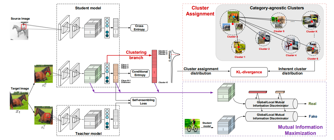
Fig. 6. Provides an overview of the SE-CC method. Image source Pan et al., 2020
Self-Ensembling
SE is similar to consistency based training where a two perturbed version of the same data point is passed to the network and the network should predict similar classification distribution over all the classes for both versions. The proposed architecture consists of a Student and a Teacher branch. Given two perturbed versions $x_t^S$ and $x_t^T$ from the same target sample $x_t$, the SE loss penalizes the difference between classification predictions of student and teacher branch.
\begin{equation} L_{SE} = ||P_{cls}^S(x_t^S) - P_{cls}^T(x_t^T)||^2 \end{equation}
During training, the student model is trained using gradient descent while the weights of the teacher model are adjusted using the Exponential moving average of student weights. The authors also make use of conditional entropy to train the student branch. Thus, overall loss becomes
\begin{equation} L_{SEC} = \sum L_{CLS}(x_s, y_s) + \sum_{x \in T} (L_{SE}(x_t) + L_{CDE}(x_t)) \end{equation}
Category Agnostic Clustering
To not group all the unknown target samples in just one class, the authors introduce a clustering branch in the student model to align its estimated cluster assignment distribution with the inherent cluster distribution among the category-agnostic clusters. We will go over what they mean by the inherent and estimated cluster distribution briefly.
The authors perform K-means clustering over the target features. The clusters so obtained reveal the underlying data distribution in the target domain i.e. its inherent cluster distribution. Next, the authors compute softmax over the cosine similarity between target samples and each cluster centroid.
\begin{equation} \overline{P_{clu}(x_t)}= \frac{e^{\gamma . cos(x_t, \mu_k)}}{\sum_{k}e^{\gamma . cos(x_t, \mu_k)}}, \mu_k=\frac{1}{|C_k|}\sum_{x_t \in C_k} x_t \end{equation}
Clustering Branch
The clustering branch is designed to predict the distribution over all category category-agnostic clusters. Depending on the input feature $x_t^S$ the clustering branch assigns it to one of the $K$ clusters and that is how we obtain the target feature’s estimated cluster assignment distribution $P^k_{clu}(x_t^S) \in \R$ via a modified softmax layer.
\begin{equation} P_{clu}^k(x_t^S) = \frac{e^{\gamma . cos(x_t^S, W_k)}}{\sum_{k}e^{\gamma . cos{x_t^S, W_k}}} \end{equation}
Here, $P_{clu}^k(x_t^S)$ represents the probability of assigning $x_t^S$ into $k$-th cluster. $W_k$ is the $k$-th row of parameter matrix $W \in \R^{K \times M}$ in the modified softmax layer, represents the cluster assignment parameter matrix for the $k$-th cluster.
To measure the similarity between the estimated cluster assignment from the clustering branch and the inherent cluster distribution obtained using $K$-means clustering, the authors have used the KL-divergence loss.
\begin{equation} L_{KL} = \sum_{x_t \in T} KL(\overline{P_{clu}(x_t)}||P_{clu}(x_t^S)) \end{equation}
The authors claim that by enforcing KL divergence, the learnt representations for target samples belonging to the known samples become aligned to the source and all the target samples retain their inherent discriminitiveness. In addition to the above practices, the authors also make use of Mutual Information both at local and global level to further enhance the learnt representations. With the above formulation, the authors achieve the best results on open-set DA tasks.
For more details, please refer to their paper mentioned in the link.
Conclusion
In the above blog post, we saw several approaches towards mitigating the domain shift between the target and source dataset in an unsupervised manner. We also explored the two types of domain adaptation namely, closed-set and open-set and saw the disadvantages of applying closed-set DA strategies for open-set DA tasks. We also discussed an improvement in the traditional open-set DA setup where minimizing the divergence between the inherent cluster distribution and the predicted cluster distribution can not only help in aligning the source and target features but also help the target features retain their inherent discriminative ness. In the next post, we will domain adaptation approaches when a few of the target samples are labelled. Such techniques fall under the purview of Few-shot domain adaptation and will hopefully prove to be an interesting read.