Building a custom OCR using pytorch
An implementation of OCR from scratch in python.
- Setting up the Data
- Defining our Model
- The CTC Loss
- The Training Loop
- Putting Everything Together
- Evaluation and testing
- Conclusion

So in this tutorial, I will give you a basic code walkthrough for building a simple OCR. OCR as might know stands for optical character recognition or in layman terms it means text recognition. Text recognition is one of the classic problems in computer vision and is still relevant today. One of the most important applications of text recognition is the digitization of old manuscripts. Physical copies of books and manuscripts are prone to degradations. With time, the printed characters start to fade. One simple way to preserve such documents is to make a digital copy of it and store it in the cloud or local hard drive which would ensure their continuance. Scanning the document or taking picture seems like a viable alternative, however if you want to perform search and retrieval or some other edit actions on the document then OCR is the way to go.Similarly, text recognition can also be used for licence plate recognition and can also be used in forensics in terms of handwriting recognition.
Okay, now that I have given you enough motivation as to why OCR is important, let me show you how you can build one. You can find the ipython notebook as well as the other dependencies in this repo. So, in case you want to run the code alongside just do a quick
git clone https://github.com/Deepayan137/Adapting-OCR
This blog assumes that you are fairly familiar with Python and Pytorch deep learning framework. If not then I will recommend you going through the Pytorch 60 minutes blitz page. It provides a nice primer on the Pytorch framework. For more details consider going through Fastai course.
So first things first, I’ll start with listing down some of the essential packages that you would need to build your first OCR. As mentioned we will be working with PyTorch 1.5 as it is one of the most efficient deep learning libraries present. The other packages are as follows:
- Matplotlib
- Tqdm
- textdistance
- lmdb
You can install them either via a pip or conda. I will also be providing a requirements.txt which you can find in my Github repo. Do a simple
pip install -r requirements and you are good to go.
Setting up the Data
We will start our project by importing the necessary libraries. But before that we need data. Now, you are free to use any data you might like (as long as it is related to documents) and for that, you might need to build your own data loader. However, in the interest of keeping things simple, we will be using a neat little package called trdg, which is a synthetic image generator for OCR. You can find all the relevant information regarding this package on its github repository. You can generate printed as well as hand-written text images and infuse them with different kinds of noise and degradation. In this project, I have used trdg to generate printed word images of a single font. You can use any font you like. Just download a .ttf file for your font and while generating the word images be sure to specify the -ft parameter as your font file.
You can generate the word images for training using the following commands:
trdg -i words.txt -c 20000 --output_dir data/train -ft your/fontfile
Here, -c refers to the number of word images you want to generate. words.txt file contains our input word vocabulary while --output_dir and -ft refer to the output and font file respectively. You can similarly generate the test word images for evaluating the performance of your OCR. However, ensure that words for training and testing are mutually exclusive to each other.
Now that we have generated the word images, let us display a few images using matlplotlib %# TODO diplay images from folder
Lets start importing the libraries that we would need to build our OCR
import os
import sys
import pdb
import six
import random
import lmdb
from PIL import Image
import numpy as np
import math
from collections import OrderedDict
from itertools import chain
import logging


import torch
import torch.nn as nn
import torch.nn.functional as F
from torch.utils.data import Dataset
from torch.utils.data import sampler
import torchvision.transforms as transforms
from torch.optim.lr_scheduler import CosineAnnealingLR, StepLR
from torch.nn.utils.clip_grad import clip_grad_norm_
from torch.utils.data import random_split

from src.utils.utils import AverageMeter, Eval, OCRLabelConverter
from src.utils.utils import EarlyStopping, gmkdir
from src.optim.optimizer import STLR
from src.utils.utils import gaussian
from tqdm import *
Next, let us create our data pipe-line. We do this by inheriting the PyTorch Dataset class. The Dataset class has few methods that we need to adhere to like the __len__ and __getitem__ method. The __len__ method returns the number of items in our dataset while __getitem_ returns the data item for the index passed. You can find more information on PyTorch Dataset class on PyTorch’s official documentation page.
You will observe that we first convert each image into grayscale and convert it into a tensor. This is followed by normalizing the images so that our input data lies within a range of [-1, 1]. We pass all such transformations into a list and later call the transforms to .Compose function provided by PyTorch. The transforms.Compose function applies each transformation in a pre-defined order.
class SynthDataset(Dataset):
    def __init__(self, opt):
        super(SynthDataset, self).__init__()
        self.path = os.path.join(opt['path'], opt['imgdir'])
        self.images = os.listdir(self.path)
        self.nSamples = len(self.images)
        f = lambda x: os.path.join(self.path, x)
        self.imagepaths = list(map(f, self.images))
       	transform_list =  [transforms.Grayscale(1),
                            transforms.ToTensor(),
                            transforms.Normalize((0.5,), (0.5,))]
        self.transform = transforms.Compose(transform_list)
        self.collate_fn = SynthCollator()

    def __len__(self):
        return self.nSamples

    def __getitem__(self, index):
        assert index <= len(self), 'index range error'
        imagepath = self.imagepaths[index]
        imagefile = os.path.basename(imagepath)
        img = Image.open(imagepath)
        if self.transform is not None:
            img = self.transform(img)
        item = {'img': img, 'idx':index}
        item['label'] = imagefile.split('_')[0]
        return item
Next, since we are going to train our model using the mini-batch gradient descent, it is essential that each image in the batch is of the same shape and size. For this, we have defined the SynthCollator class which initially finds the image with maximum width in the batch and then proceeds to pad the remaining images to have the same width. You migh wonder as to why we are not concerned with the height, it is because while generating the images using the trdg package, I had fixed the height to 32 pixels.
class SynthCollator(object):

    def __call__(self, batch):
        width = [item['img'].shape[2] for item in batch]
        indexes = [item['idx'] for item in batch]
        imgs = torch.ones([len(batch), batch[0]['img'].shape[0], batch[0]['img'].shape[1],
                           max(width)], dtype=torch.float32)
        for idx, item in enumerate(batch):
            try:
                imgs[idx, :, :, 0:item['img'].shape[2]] = item['img']
            except:
                print(imgs.shape)
        item = {'img': imgs, 'idx':indexes}
        if 'label' in batch[0].keys():
            labels = [item['label'] for item in batch]
            item['label'] = labels
        return item
Defining our Model
Now we proceed to define our model. We use the CNN-LSTM based architecture which was proposed by Shi et.al. in their excellent paper An End-to-End Trainable Neural Network for Image-based Sequence Recognition and Its Application to Scene Text Recognition. The authors used it for scene-text recognition and showed via extensive experimentation that they were able to achieve significant gains in accuracy compared to all other existing methods at that time.
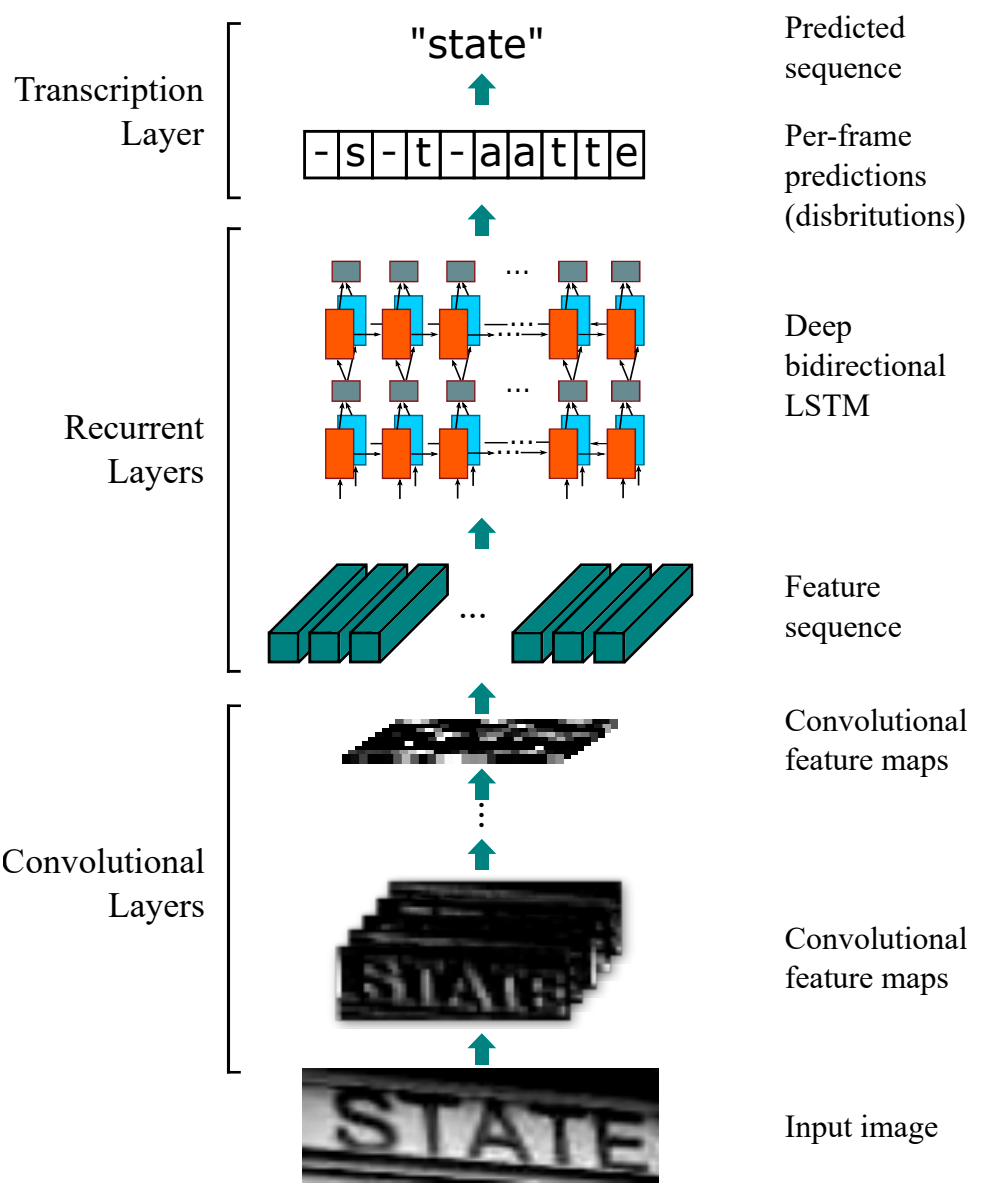
The figure above shows the architecture used in the paper. The authors used a 7 layered Convolution network with BatchNorm and ReLU. This was followed by a stacked RNN network consisting of two Bidirectional LSTM layers. The convolution layers acted as a feature extractor while the LSTMs layers act as sequence classifiers. The LSTM layers output the probability associated with each output class at each time step Further details can be found in their paper and I strongly suggest you go through it for a better understanding.
The below code snippet is taken from this github repository which provides a Pytorch implementation of their code.
class BidirectionalLSTM(nn.Module):

    def __init__(self, nIn, nHidden, nOut):
        super(BidirectionalLSTM, self).__init__()
        self.rnn = nn.LSTM(nIn, nHidden, bidirectional=True)
        self.embedding = nn.Linear(nHidden * 2, nOut)
    def forward(self, input):
        self.rnn.flatten_parameters()
        recurrent, _ = self.rnn(input)
        T, b, h = recurrent.size()
        t_rec = recurrent.view(T * b, h)
        output = self.embedding(t_rec)  # [T * b, nOut]
        output = output.view(T, b, -1)
        return output

class CRNN(nn.Module):

    def __init__(self, opt, leakyRelu=False):
        super(CRNN, self).__init__()

        assert opt['imgH'] % 16 == 0, 'imgH has to be a multiple of 16'

        ks = [3, 3, 3, 3, 3, 3, 2]
        ps = [1, 1, 1, 1, 1, 1, 0]
        ss = [1, 1, 1, 1, 1, 1, 1]
        nm = [64, 128, 256, 256, 512, 512, 512]

        cnn = nn.Sequential()

        def convRelu(i, batchNormalization=False):
            nIn = opt['nChannels'] if i == 0 else nm[i - 1]
            nOut = nm[i]
            cnn.add_module('conv{0}'.format(i),
                           nn.Conv2d(nIn, nOut, ks[i], ss[i], ps[i]))
            if batchNormalization:
                cnn.add_module('batchnorm{0}'.format(i), nn.BatchNorm2d(nOut))
            if leakyRelu:
                cnn.add_module('relu{0}'.format(i),
                               nn.LeakyReLU(0.2, inplace=True))
            else:
                cnn.add_module('relu{0}'.format(i), nn.ReLU(True))

        convRelu(0)
        cnn.add_module('pooling{0}'.format(0), nn.MaxPool2d(2, 2))  # 64x16x64
        convRelu(1)
        cnn.add_module('pooling{0}'.format(1), nn.MaxPool2d(2, 2))  # 128x8x32
        convRelu(2, True)
        convRelu(3)
        cnn.add_module('pooling{0}'.format(2),
                       nn.MaxPool2d((2, 2), (2, 1), (0, 1)))  # 256x4x16
        convRelu(4, True)
        convRelu(5)
        cnn.add_module('pooling{0}'.format(3),
                       nn.MaxPool2d((2, 2), (2, 1), (0, 1)))  # 512x2x16
        convRelu(6, True)  # 512x1x16
        self.cnn = cnn
        self.rnn = nn.Sequential()
        self.rnn = nn.Sequential(
            BidirectionalLSTM(opt['nHidden']*2, opt['nHidden'], opt['nHidden']),
            BidirectionalLSTM(opt['nHidden'], opt['nHidden'], opt['nClasses']))


    def forward(self, input):
        # conv features
        conv = self.cnn(input)
        b, c, h, w = conv.size()
        assert h == 1, "the height of conv must be 1"
        conv = conv.squeeze(2)
        conv = conv.permute(2, 0, 1)  # [w, b, c]
        # rnn features
        output = self.rnn(conv)
        output = output.transpose(1,0) #Tbh to bth
        return output
The CTC Loss
Cool, now that we have our data and model pipeline ready, it is time to define our loss function which in our case is the CTC loss function. We will be using PyTorch’s excellent CTC implementation. CTC stands for Connectionist Temporal Classification and was proposed by Alex Graves in his paper Connectionist Temporal Classification: Labelling Unsegmented Sequence Data with Recurrent Neural Networks.
Honestly, the above work has been a gamechanger for many sequences based tasks like speech and text recognition. For all the sequence-based tasks it is important for the input and output labels to be properly aligned. Proper alignment leads to efficient loss computation between the network predictions and expected output. In segmentation based approaches i.e. when the input word or line has been segmented into its constituent characters, there exists a direct one-to-one mapping between the segmented images of characters and the output labels. However, as you might imagine obtaining such segmentations for each character can be a very tedious and time-consuming task. Thus, CTC based transcription layers have become the de-facto choice for OCRs and speech recognition module since it allows loss computation without explicit mapping between the input and output. The CTC layer takes the output from the LSTMs and computes a score with all possible alignments of the target label. The OCR is then trained to predict a sequence which maximizes the sum of all such scores.
If you want more thorough details regarding the CTC layer I would suggest you go through the following blogs and lecture video
class CustomCTCLoss(torch.nn.Module):
    # T x B x H => Softmax on dimension 2
    def __init__(self, dim=2):
        super().__init__()
        self.dim = dim
        self.ctc_loss = torch.nn.CTCLoss(reduction='mean', zero_infinity=True)

    def forward(self, logits, labels,
            prediction_sizes, target_sizes):
        EPS = 1e-7
        loss = self.ctc_loss(logits, labels, prediction_sizes, target_sizes)
        loss = self.sanitize(loss)
        return self.debug(loss, logits, labels, prediction_sizes, target_sizes)

    def sanitize(self, loss):
        EPS = 1e-7
        if abs(loss.item() - float('inf')) < EPS:
            return torch.zeros_like(loss)
        if math.isnan(loss.item()):
            return torch.zeros_like(loss)
        return loss

    def debug(self, loss, logits, labels,
            prediction_sizes, target_sizes):
        if math.isnan(loss.item()):
            print("Loss:", loss)
            print("logits:", logits)
            print("labels:", labels)
            print("prediction_sizes:", prediction_sizes)
            print("target_sizes:", target_sizes)
            raise Exception("NaN loss obtained. But why?")
        return loss
The Training Loop
The above code snippet builds a wrapper around pytorch’s CTC loss function. Basically, what it does is that it computes the loss and passes it through an additional method called debug, which checks for instances when the loss becomes Nan.
Shout out to Jerin Philip for this code.
Till now we have defined all the important components which we need to build our OCR. We have defined the data pipeline, our model as well as the loss function. Now its time to talk abot our training loop. The below code might look a bit cumbersome but it provides a nice abstraction which is quite intuitive and easy to use. The code is based on pytorch lighning’s bolier plate template with few modifications of my own. :P
I will give a basic overview of what it does. Feel free to inspect each method using python debugger. The OCRTrainer class takes in the training and validation data. It also takes in the loss function, optimizer and the number of epochs it needs to train the model. The train and validation loader method returns the data loader for the train and validation data. The run_batch method does one forward pass for a batch of image-label pairs. It returns the loss as well as the character and word accuracy. Next, we have the step function which performs the backpropagation, calculates the gradients and updates the parameters for each batch of data. Besides we also have the training_end and validation_end methods that calculate the mean loss and accuracy for all the batchs after the completion of one single epoch
The methods defined are quite simple and I hope you will get the hang of it in no time.
class OCRTrainer(object):
    def __init__(self, opt):
        super(OCRTrainer, self).__init__()
        self.data_train = opt['data_train']
        self.data_val = opt['data_val']
        self.model = opt['model']
        self.criterion = opt['criterion']
        self.optimizer = opt['optimizer']
        self.schedule = opt['schedule']
        self.converter = OCRLabelConverter(opt['alphabet'])
        self.evaluator = Eval()
        print('Scheduling is {}'.format(self.schedule))
        self.scheduler = CosineAnnealingLR(self.optimizer, T_max=opt['epochs'])
        self.batch_size = opt['batch_size']
        self.count = opt['epoch']
        self.epochs = opt['epochs']
        self.cuda = opt['cuda']
        self.collate_fn = opt['collate_fn']
        self.init_meters()

    def init_meters(self):
        self.avgTrainLoss = AverageMeter("Train loss")
        self.avgTrainCharAccuracy = AverageMeter("Train Character Accuracy")
        self.avgTrainWordAccuracy = AverageMeter("Train Word Accuracy")
        self.avgValLoss = AverageMeter("Validation loss")
        self.avgValCharAccuracy = AverageMeter("Validation Character Accuracy")
        self.avgValWordAccuracy = AverageMeter("Validation Word Accuracy")

    def forward(self, x):
        logits = self.model(x)
        return logits.transpose(1, 0)

    def loss_fn(self, logits, targets, pred_sizes, target_sizes):
        loss = self.criterion(logits, targets, pred_sizes, target_sizes)
        return loss

    def step(self):
        self.max_grad_norm = 0.05
        clip_grad_norm_(self.model.parameters(), self.max_grad_norm)
        self.optimizer.step()

    def schedule_lr(self):
        if self.schedule:
            self.scheduler.step()

    def _run_batch(self, batch, report_accuracy=False, validation=False):
        input_, targets = batch['img'], batch['label']
        targets, lengths = self.converter.encode(targets)
        logits = self.forward(input_)
        logits = logits.contiguous().cpu()
        logits = torch.nn.functional.log_softmax(logits, 2)
        T, B, H = logits.size()
        pred_sizes = torch.LongTensor([T for i in range(B)])
        targets= targets.view(-1).contiguous()
        loss = self.loss_fn(logits, targets, pred_sizes, lengths)
        if report_accuracy:
            probs, preds = logits.max(2)
            preds = preds.transpose(1, 0).contiguous().view(-1)
            sim_preds = self.converter.decode(preds.data, pred_sizes.data, raw=False)
            ca = np.mean((list(map(self.evaluator.char_accuracy, list(zip(sim_preds, batch['label']))))))
            wa = np.mean((list(map(self.evaluator.word_accuracy, list(zip(sim_preds, batch['label']))))))
        return loss, ca, wa

    def run_epoch(self, validation=False):
        if not validation:
            loader = self.train_dataloader()
            pbar = tqdm(loader, desc='Epoch: [%d]/[%d] Training'%(self.count,
                self.epochs), leave=True)
            self.model.train()
        else:
            loader = self.val_dataloader()
            pbar = tqdm(loader, desc='Validating', leave=True)
            self.model.eval()
        outputs = []
        for batch_nb, batch in enumerate(pbar):
            if not validation:
                output = self.training_step(batch)
            else:
                output = self.validation_step(batch)
            pbar.set_postfix(output)
            outputs.append(output)
        self.schedule_lr()
        if not validation:
            result = self.train_end(outputs)
        else:
            result = self.validation_end(outputs)
        return result

    def training_step(self, batch):
        loss, ca, wa = self._run_batch(batch, report_accuracy=True)
        self.optimizer.zero_grad()
        loss.backward()
        self.step()
        output = OrderedDict({
            'loss': abs(loss.item()),
            'train_ca': ca.item(),
            'train_wa': wa.item()
            })
        return output

    def validation_step(self, batch):
        loss, ca, wa = self._run_batch(batch, report_accuracy=True, validation=True)
        output = OrderedDict({
            'val_loss': abs(loss.item()),
            'val_ca': ca.item(),
            'val_wa': wa.item()
            })
        return output

    def train_dataloader(self):
        # logging.info('training data loader called')
        loader = torch.utils.data.DataLoader(self.data_train,
                batch_size=self.batch_size,
                collate_fn=self.collate_fn,
                shuffle=True)
        return loader

    def val_dataloader(self):
        # logging.info('val data loader called')
        loader = torch.utils.data.DataLoader(self.data_val,
                batch_size=self.batch_size,
                collate_fn=self.collate_fn)
        return loader

    def train_end(self, outputs):
        for output in outputs:
            self.avgTrainLoss.add(output['loss'])
            self.avgTrainCharAccuracy.add(output['train_ca'])
            self.avgTrainWordAccuracy.add(output['train_wa'])

        train_loss_mean = abs(self.avgTrainLoss.compute())
        train_ca_mean = self.avgTrainCharAccuracy.compute()
        train_wa_mean = self.avgTrainWordAccuracy.compute()

        result = {'train_loss': train_loss_mean, 'train_ca': train_ca_mean,
        'train_wa': train_wa_mean}
        # result = {'progress_bar': tqdm_dict, 'log': tqdm_dict, 'val_loss': train_loss_mean}
        return result

    def validation_end(self, outputs):
        for output in outputs:
            self.avgValLoss.add(output['val_loss'])
            self.avgValCharAccuracy.add(output['val_ca'])
            self.avgValWordAccuracy.add(output['val_wa'])

        val_loss_mean = abs(self.avgValLoss.compute())
        val_ca_mean = self.avgValCharAccuracy.compute()
        val_wa_mean = self.avgValWordAccuracy.compute()

        result = {'val_loss': val_loss_mean, 'val_ca': val_ca_mean,
        'val_wa': val_wa_mean}
        return result
Putting Everything Together
Finally, we have the Learner class. It implements a couple more methods like the save and load. It also tracks the losses and saves them in a csv file. This comes in handy if we want to analyze the behaviour of our training and validation loops. It initializes our OCRTrainer module with the necessary hyperparameters and later calls the fit method which runs the training loop.
Besides these methods, we have a bunch of helper methods like the OCRLabel_converter, Eval and Averagemeter. I am not including them in this notebook, instead, I have written them in utils.py file and I am importing them from there. In case you want to take a peek, feel free to tinker with the utils.py file. All the necessary documentation is provided in the file itself.
class Learner(object):
    def __init__(self, model, optimizer, savepath=None, resume=False):
        self.model = model
        self.optimizer = optimizer
        self.savepath = os.path.join(savepath, 'best.ckpt')
        self.cuda = torch.cuda.is_available()
        self.cuda_count = torch.cuda.device_count()
        if self.cuda:
            self.model = self.model.cuda()
        self.epoch = 0
        if self.cuda_count > 1:
            print("Let's use", torch.cuda.device_count(), "GPUs!")
            self.model = nn.DataParallel(self.model)
        self.best_score = None
        if resume and os.path.exists(self.savepath):
            self.checkpoint = torch.load(self.savepath)
            self.epoch = self.checkpoint['epoch']
            self.best_score=self.checkpoint['best']
            self.load()
        else:
            print('checkpoint does not exist')

    def fit(self, opt):
        opt['cuda'] = self.cuda
        opt['model'] = self.model
        opt['optimizer'] = self.optimizer
        logging.basicConfig(filename="%s/%s.csv" %(opt['log_dir'], opt['name']), level=logging.INFO)
        self.saver = EarlyStopping(self.savepath, patience=15, verbose=True, best_score=self.best_score)
        opt['epoch'] = self.epoch
        trainer = OCRTrainer(opt)

        for epoch in range(opt['epoch'], opt['epochs']):
            train_result = trainer.run_epoch()
            val_result = trainer.run_epoch(validation=True)
            trainer.count = epoch
            info = '%d, %.6f, %.6f, %.6f, %.6f, %.6f, %.6f'%(epoch, train_result['train_loss'],
                val_result['val_loss'], train_result['train_ca'],  val_result['val_ca'],
                train_result['train_wa'], val_result['val_wa'])
            logging.info(info)
            self.val_loss = val_result['val_loss']
            print(self.val_loss)
            if self.savepath:
                self.save(epoch)
            if self.saver.early_stop:
                print("Early stopping")
                break

    def load(self):
        print('Loading checkpoint at {} trained for {} epochs'.format(self.savepath, self.checkpoint['epoch']))
        self.model.load_state_dict(self.checkpoint['state_dict'])
        if 'opt_state_dict' in self.checkpoint.keys():
            print('Loading optimizer')
            self.optimizer.load_state_dict(self.checkpoint['opt_state_dict'])

    def save(self, epoch):
        self.saver(self.val_loss, epoch, self.model, self.optimizer)
Defining the hyperparameters
We have come a long way now and there is just one more hurdle to cross before we can start training our model. We begin by defining our vocabulary i.e. the alphabets which serve as the output classes for our model. We define a suitable name for this experiment which will also serve as the folder name where the checkpoints and log files will be stored. We also define the hyper-parameters like the batch size, learning rate, image height, number of channels etc.
Then we initialize our Dataset class and split the data into train and validation. We then proceed to initialize our Model and CTCLoss and finally call the learner.fit function.
Once the training is over we can find the saved model in the checkpoints/name folder. We may load the model and evaluate its performance on the test data or finetune it on some other data.
alphabet = """Only thewigsofrcvdampbkuq.$A-210xT5'MDL,RYHJ"ISPWENj&BC93VGFKz();#:!7U64Q8?+*ZX/%"""
args = {
    'name':'exp1',
    'path':'data',
    'imgdir': 'train',
    'imgH':32,
    'nChannels':1,
    'nHidden':256,
    'nClasses':len(alphabet),
    'lr':0.001,
    'epochs':4,
    'batch_size':32,
    'save_dir':'checkpoints',
    'log_dir':'logs',
    'resume':False,
    'cuda':False,
    'schedule':False

}

data = SynthDataset(args)
args['collate_fn'] = SynthCollator()
train_split = int(0.8*len(data))
val_split = len(data) - train_split
args['data_train'], args['data_val'] = random_split(data, (train_split, val_split))
print('Traininig Data Size:{}\nVal Data Size:{}'.format(
    len(args['data_train']), len(args['data_val'])))
args['alphabet'] = alphabet
model = CRNN(args)
args['criterion'] = CustomCTCLoss()
savepath = os.path.join(args['save_dir'], args['name'])
gmkdir(savepath)
gmkdir(args['log_dir'])
optimizer = torch.optim.Adam(model.parameters(), lr=args['lr'])
learner = Learner(model, optimizer, savepath=savepath, resume=args['resume'])
learner.fit(args)
Evaluation and testing
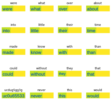
Once, our model is trained we can evaluate its performance on the test data. I have written a separate function get_accuracy which takes in the trained model and the test data and performs a forward pass which gives us the logits. Once we get the logits we perform an argmax operation at each time step which we treat as our predicted class. Finally, we perform a decoding operation which converts the token ids to their respective class ids. We compare the predicted string with its corresponding ground-truth which gives us the accuracy. We do it for all the images in our test data and take the mean accuracy.
We also display random 20 images from our test data with its corresponding predicted label using the Matplotlib library
import matplotlib.pyplot as plt
from torchvision.utils import make_grid
device = torch.device("cuda:0" if torch.cuda.is_available() else "cpu")
def get_accuracy(args):
    loader = torch.utils.data.DataLoader(args['data'],
                batch_size=args['batch_size'],
                collate_fn=args['collate_fn'])
    model = args['model']
    model.eval()
    converter = OCRLabelConverter(args['alphabet'])
    evaluator = Eval()
    labels, predictions, images = [], [], []
    for iteration, batch in enumerate(tqdm(loader)):
        input_, targets = batch['img'].to(device), batch['label']
        images.extend(input_.squeeze().detach())
        labels.extend(targets)
        targets, lengths = converter.encode(targets)
        logits = model(input_).transpose(1, 0)
        logits = torch.nn.functional.log_softmax(logits, 2)
        logits = logits.contiguous().cpu()
        T, B, H = logits.size()
        pred_sizes = torch.LongTensor([T for i in range(B)])
        probs, pos = logits.max(2)
        pos = pos.transpose(1, 0).contiguous().view(-1)
        sim_preds = converter.decode(pos.data, pred_sizes.data, raw=False)
        predictions.extend(sim_preds)

#     make_grid(images[:10], nrow=2)
    fig=plt.figure(figsize=(8, 8))
    columns = 4
    rows = 5
    for i in range(1, columns*rows +1):
        img = images[i]
        img = (img - img.min())/(img.max() - img.min())
        img = np.array(img * 255.0, dtype=np.uint8)
        fig.add_subplot(rows, columns, i)
        plt.title(predictions[i])
        plt.axis('off')
        plt.imshow(img)
    plt.show()
    ca = np.mean((list(map(evaluator.char_accuracy, list(zip(predictions, labels))))))
    wa = np.mean((list(map(evaluator.word_accuracy_line, list(zip(predictions, labels))))))
    return ca, wa
args['imgdir'] = 'test'
args['data'] = SynthDataset(args)
resume_file = os.path.join(args['save_dir'], args['name'], 'best.ckpt')
if os.path.isfile(resume_file):
    print('Loading model %s'%resume_file)
    checkpoint = torch.load(resume_file)
    model.load_state_dict(checkpoint['state_dict'])
    args['model'] = model
    ca, wa = get_accuracy(args)
    print("Character Accuracy: %.2f\nWord Accuracy: %.2f"%(ca, wa))
else:
    print("=> no checkpoint found at '{}'".format(save_file))
    print('Exiting')
  0%|          | 0/2 [00:00<?, ?it/s]

Loading model checkpoints/exp1/best.ckpt


100%|██████████| 2/2 [00:00<00:00,  2.25it/s]
Character Accuracy: 98.89
Word Accuracy: 98.03
Conclusion
In this blog we looked at how we can build an OCR from scratch using PyTorch. For this we defined the three basic module i.e. the data module, the model and a custom loss fucntion. We then tied a wrapper around the modules in the form of a OCRTrainer class which handles the forward and backward propadation as well as the accuracies. We also defined our Learner class which contains the fit method which initilizes the Trainer class and starts training OCR model and later saves it. Finally we tested our model on a heldout set and evaluated its performance in terms of Character and Word accuracy.